


In February 2019, I was first introduced to the problem golf. At what angle should you lift a golf ball into the air such that it has the maximum range during a strike? 45° ?
Obviously, to complicate matters more, we should include parameters such as spin and air density. Up until this point in my studies, air resistance was always an assumption. It was never something that actually had a quantifiable structure...until now.
__________________________________________________________________________________________
The primary focus of this investigation was to explore the key elements influencing the trajectory of a golf ball during its flights. By examining diverse weather conditions in Singapore, Scotland, and Bolivia, and considering fundamental principles of physics, computer modelling was employed to determine the optimal loft angles for achieving maximum range.
1. Introduction
The objective of a golf drive is to maximize the ball's coverage distance. In an ideal scenario with only gravity as the influencing force, the ball follows a straightforward parabolic curve, suggesting an optimal loft angle of 45°. However, real-world complexities, including factors such as air resistance, ball spin, and surface texture, significantly impact the ball's flight. Consequently, assumptions were made, and key factors were identified to streamline the analysis.
2. Assumptions
Various assumptions were adopted, including a clubface velocity of 47.8 m/s at impact, a rigid and uniform golf ball with specific characteristics, constant driver head mass, fixed launch and loft angles, and unchanging shaft properties during swing. Additionally, the ball's spin rate and drag coefficient were considered, while factors like wind conditions were excluded for simplification.
3. Underlying Factors
F_dx = -(0.5)*air_dens*(vx)**2*C_d*r**2*pi
Drag: The drag force acting on the golf ball, caused by its movement through air, was explored. The drag force formula incorporated factors like the coefficient of drag, air density, cross-sectional area, and velocity, affecting the ball's motion contrary to its direction.
Lift: The lift force, generated by the ball's spin during impact with the clubhead, was investigated. The loft angle played a crucial role in determining the rate of spin, affecting the force acting perpendicularly upward to the ball's motion.

v = ((1+e)*((1+(mu**2))**.5)*v_club*cos(angle*pi/180))/(1+(m/M))
F_my = (0.5)*air_dens*(vy)**2*C_m*r**2*pi
C_m = 0.533333*(v_rot/v)+0.1
Texture: The impact of dimples on the golf ball's aerodynamics was discussed, emphasizing their role in minimizing drag and maximizing lift. The specific characteristics of dimples were acknowledged, but the model utilized predetermined coefficients without delving into various dimple configurations.
4. Inputs and Outputs
The Python program's constants and assumed values were outlined, with air density recognized as a vital factor influencing the ball's trajectory. The program's execution involved user inputs for the Open location, angle range, and precision, producing graphs depicting vertical and horizontal displacement for each tested angle.
5. Results
Graphs showcasing vertical against horizontal displacement for various loft angles were plotted and analysed for each location (Singapore, Scotland, and Bolivia). The optimum loft angles, associated with maximum range, were identified for each location:


Singapore: Optimum loft angle of 28.8°, achieving a range of 218m.
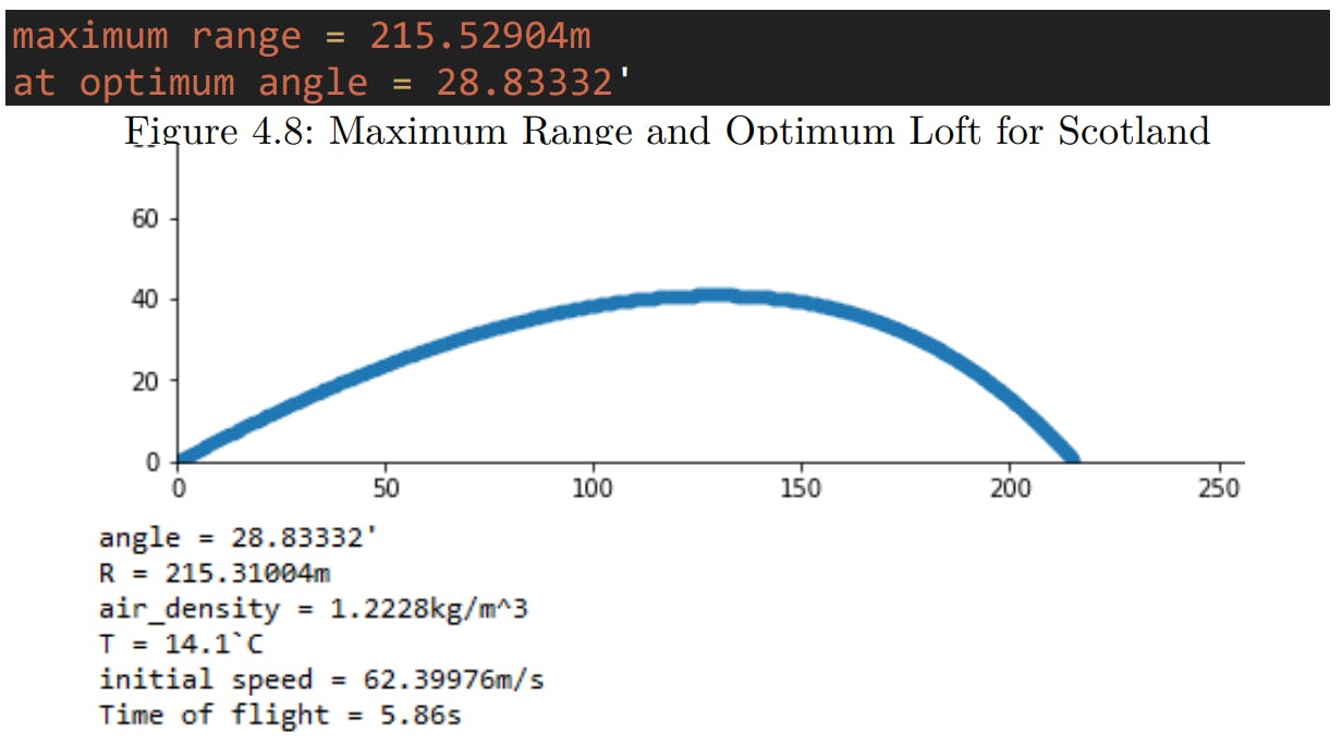
Scotland: Optimum loft angle of 28.8°, yielding a range of 215m.
Bolivia: Optimum loft angle of 28.8°, resulting in a range of 212m.
Response
Results for Various Locations
The Singapore Open (17th-20th January 2019)
In Singapore during January 2019, diverse weather conditions were observed.
Weather in Singapore, January 2019:
Average: 29.44°C (High), 27.13°C (Low), 1029.44 mbar (Pressure), 79% (Humidity)
The average temperature (T_Sing), pressure (P_t_Sing), and humidity (humid_Sing) were calculated as 28.28°C, 1.02944, and 0.79, respectively.

The Scottish Open (8th-14th July 2019)
Monthly Averages for July:
Average: 14.1°C (Temperature), 1012.66 mbar (Pressure), 84.8% (Humidity)
For Scotland, T_Scot, P_t_Scot, and humid_Scot were determined as 14.1°C, 1.01266 bar, and 0.848, respectively.
The Bolivian Open (August 2019)
The weather conditions in Bolivia during August are depicted:
Monthly Averages for August:
Average: 14.1°C (Temperature), 1012.66 mbar (Pressure), 58.1% (Humidity)
For Bolivia, T_Boli, P_t_Boli, and humid_Boli were determined as 3.2°C, 1.02007 bar, and 0.581, respectively.

Using Equation for Air Density, the air density was computed for each location.
Final Results
| Location | Air Density (kgm^-3) | Maximum Range (m) | Optimum Loft (°) |
| Singapore | 1.1793 | 217.9983 | 28.84461 |
| Scotland | 1.2228 | 215.52904 | 28.83332 |
| Bolivia | 1.2837 | 212.24216 | 28.76608 |
Results from Model
6. Real-World Applications
Despite assuming horizontal incident club head velocity, real-world golf swings involve a slightly downward strike for optimal ball-clubface contact (Cross and Dewhurst, 2018). This alters the projection angle, impacting both carry and range.
The outgoing ball speed (v2) is influenced by factors like club speed (v1), coefficient of restitution (e), frictional force (μ), and launch angle (A).
Variability in swing speed and clubhead flexion during impact introduce uncertainties into the model. The dynamic nature of these factors could potentially affect the ball's velocity and maximum range.
The assumption of constant spin neglects the impact of ball characteristics, club interaction, and wind conditions. Real-world scenarios involve varied spin rates influenced by factors like ball composition, club impact location, and wind effects.
Acknowledging these real-world complexities, future models could strive for a more nuanced understanding by considering additional variables and experimental data from wind tunnel tests. This would enhance the accuracy and applicability of the model to diverse golfing conditions.
__________________________________________________________________________________________
I would further like to thank Matthew Deighan, Soo Bynn, Lee Kenneth Ng and Isobel Reid for their research, investigations and ideas which supported the success of this group project.
The following includes the code which achieves the following results. I would like to thank Gregory Dritschel, who has not only had the patients but the heart to help me tackle this problem while I was in 1st year Physics and he was in 2nd year direct entry to Maths. I've came along way in my simulation and programming skills, but I believe that the spirit of its interest first began with this problem.
#Open in Anaconda- Spyder or any other model-supported Python system

from numpy import *
from pylab import *

print("      ")
print("Name: Clark Gray and Gregory Dritschel")
print("")

Range_of_Driver = 275

T_Boli = 3.4
P_t_Boli = 1020.07*10**-3
humid_Boli = 0.581
air_dens_Boli = 1.2837

T_Sing = 28.281
P_t_Sing = 1.009185*10**-3
humid_Sing = 0.79
air_dens_Sing = 1.1793

T_Scot = 14.1
P_t_Scot = 1.01266*10**-3
humid_Scot = 0.848
air_dens_Scot = 1.2228

#Above we have our weather conditions for each location. The pressure
#is calculated using an online pressure calculator implementing humid air

print("Enter location and time of")
print("the Open using the keys:")
print("                         " )
print("Scot     ====     Scotland")
print("Boli     ====     Bolivia" )
print("Sing     ====     Singapore")
#Takes user input for each location
while True:
    loca = input("Where is the Open?: ")
    if loca == "Sing":
        air_dens = air_dens_Sing
        T = 28.281
        print("The Singapore Open (held 17-20 January, 2019)")
        break
    elif loca == "Scot":
        air_dens = air_dens_Scot
        T = 14.1
        print("The Scottish Open (held at The Renaissance Club (East Lothian),  July 8-14, 2019)")
        break
    elif loca == "Boli":
        print("A potential Bolivian Open at La Paz Golf Club, Bolivia (alongside Lake Titicaca)  in August 2019")
        air_dens = air_dens_Boli
        T = 3.4
        break
    #assigns air density to value at location
    else:
        print("Invalid Location")

if loca == "Sing":
    air_dens = 1.1793
    T = 28.281
elif loca == "Scot":
    air_dens = 1.2228
    T = 14.1
elif loca == "Boli":
    air_dens = 1.2837
    T = 3.4
else:
    print("Invalid Location-Use keys")

g = -9.8
#acceleration due to gravity
r = 0.021
#radiius of the ball
rpm = 3600
#revolutions per minute
v_rot = r*2*pi*rpm/60**2
#tangential velocity of rotaional motion
v_club = 47.8333
#velocity of club

mu = 0.035
e = 0.83
#constants for velocity of ball equation (line 12)
C_d = 0.25
#coeffiecient of drag
#Defining constants and assumed values

#Running air density values for each location by user's input

m = 0.04593
#mass of ball
M = 0.2
#mass of club
angle = 10
#defining mass of golf ball, mass of golf driver, initial angle of launch,
Rsol = []
angles = []
angles.append(angle)

angle_lower = float(input("Enter lower angle (recommended: 28) : "))
angle_upper = float(input("Enter upper angle (recommended: 29) : "))
print("This exacutes the programme bewteen a range of two sets of degrees)")
print("           ")
print("Note that as precisison increases, the number and time to iterate")
print("each graph increases exponentially.It is advised that to achieve greater")
print("sig figs for the final solution, adjust the lower and upper angles while")
print("increasing the precision. This prevents overloading the script.")
precision_C = int(input("Enter magnitude of precision (recommended : 10 - 3000): "))
#chose the degree of precision for your range of angles
num_runs = float(precision_C*(angle_upper -angle_lower)) - 1
for angle in range(int(angle_lower*precision_C),int(angle_upper*precision_C)):
    #Above exacutes the code bewteen a range of two sets of degrees, with
    # a chosen extreme of significant figures. Both upper and lower angle limit
    #must have the same number of sig figs
    angle = angle/precision_C
    #Note that as precisison_C increases, the number and time to iterate
    #each graph increases exponentially.It is advised that to achieve greater
    #sig figs the final solution, adjusting the lower and upper angles while
    # increasing the precision_C. This prevents overloading the script.

    angles.append(angle)
    x = 0
    y = 0
    v = ((1+e)*((1+(mu**2))**.5)*v_club*cos(angle*pi/180))/(1+(m/M))

    #Equation of initial ball speed as a function of angle of loft,
    #and driver mass and speed, mass of ball
    C_m = 0.533333*(v_rot/v)+0.1
    #Magnus (Lift) coefficient as function of ball's rotational velocity and
    #projectile speed
    vx = v*cos(angle*pi/180)
    vy = v*sin(angle*pi/180)
    #Dividing x, y components of velocity with respect to launch angle

    xsol = []
    ysol = []
    #creates a set to store x, y positions
    xsol.append(x)
    ysol.append(y)

    vxsol = []
    vysol = []
    #creates a set to store x, y components of velocity
    vxsol.append(vx)
    vysol.append(vy)
    #setting up the arrays for storing x, y positions and velocity in the x
    # and y direction
    t = 0

    for i in range(1000):
        ts = 0.01
        #time step assigned
        t = t + ts
        if vy>=0:#before the ball reaches it's maximum height
            F_dy = -(0.5)*air_dens*(vy)**2*C_d*r**2*pi
        else: #after the ball reaches its max height
            F_dy = (0.5)*air_dens*(vy)**2*C_d*r**2*pi

        F_dx = -(0.5)*air_dens*(vx)**2*C_d*r**2*pi
        #Force of drag for each x, y component
        F_mx = -(0.5)*air_dens*(vx)**2*C_m*r**2*pi
        if vy>=0:#same for the lift force due to spin
            F_mx = (0.5)*air_dens*(vx)**2*C_m*r**2*pi
        else:
            F_mx = -(0.5)*air_dens*(vx)**2*C_m*r**2*pi

        F_my = (0.5)*air_dens*(vy)**2*C_m*r**2*pi

        ax = (F_dx+F_mx)/m
        ay = g + (F_dy+F_my)/m
        #acceleration of the ball by Newton's 2nd Law of Motion
        vx = vxsol[i] + ax*ts
        vy = vysol[i] + ay*ts
        #by v = u + at, iterate over discrete time steps
        x = xsol[i] + vx*ts
        y = ysol[i] + vy*ts
        #adding the positions in the x,y components
        if y<0 :
            R = (x+xsol[i-1])/2
            Rsol.append(R)
            break
        #once the ball has negative height, (below the ground) , calculate the
        #range by taking the average of the x-values just above and below the
        #x-axis
        #print(i,round(x, 5),round(y, 5))
        xsol.append(x)
        ysol.append(y)
        #adding the ball's position to the position array wrt the the
        #previous value
        vxsol.append(vx)
        vysol.append(vy)
         #add the ball's velocty to the velocity array for each component wrt
        #its acceleretion at
        #each time step

        #print(round(vx,5), round(vy,5),round(x,5), round(y, 5))
        #The above code is commented-out, prints the velocity in the x and y
        #direction as well as the x and y position to 5 sig figs

    if num_runs <=500:
        figure(figsize=(12, 3.16))
        scatter(xsol,ysol, s=20)
        xlim(0, 380)
        ylim(0,100)
        show()
        #organsing the dimensions and display of graph. Advised to comment-out
        #when dealing with huge number of graphs.
    if num_runs <=1000:
        #ensures that data for each run is not printed if the load is too high
        #allows code to execute directly to solution.
        print("angle = " + str(angle) + "'")
        print("R = " + str(round(R,5)) + "m")
        print("air_density = " + str(round(air_dens, 5)) + "kg/m^3")
        print("T = " + str(T) +"`C")
        print("initial speed = " + str(round(v,5)) + "m/s")
        print("Time of flight = " + str(round(t,4)) + "s")
        # for each graph, display the launch angle, the range, air density,
        #temperature, initial speed and time of flight

maxrange = 0
for R in Rsol:
    if R>=maxrange:
        maxrange = R
#Checker for defining max range
for i in range(len(Rsol)):
    if Rsol[i] >= maxrange:
        maxrange = Rsol[i]
        maxangle = angles[i]
#By defining max range, the cotrresponding angle can be located
print("                     ")
print("Final solutions for: " + loca)
print("maximum range = " + str(round(maxrange, 5)) + "m")
print(" at optimum angle = " + str(maxangle)+"'")
#Display final solutions for particular location